RMSProp: Why Every Parameter Shouldn't Take the Same Step

Two weights. One learning rate.

One weight barely moves. The other keeps overshooting.

We can lower the learning rate to calm the second weight. But then the first moves even more slowly.

What if each parameter used its own scale for the update?

The same learning rate already produces different steps

Ordinary gradient descent uses:

$$w_i\leftarrow w_i-\alpha g_i$$

The subscript $i$ selects one parameter. The gradient $g_i$ tells us how the loss changes with that parameter.

If $\alpha =0.01$ and the gradients are 1 and 100, the update magnitudes are 0.01 and 1.

So the title needs one clarification: gradient descent does not literally move every parameter the same distance. It applies the same multiplier to every gradient.

RMSProp changes that multiplier using each parameter’s recent gradient history.

Momentum remembers direction. What remembers size?

In the previous post, Momentum averaged signed gradients.

That is useful for direction. But consider:

$$10,-10,10,-10$$

The ordinary average is zero. The gradients themselves are not small.

If we want a measure of size, positive and negative values should not cancel. Squaring solves this:

$$100,100,100,100$$

Maintain an exponentially weighted average of those squares:

$$s_t=\beta s_{t-1}+(1-\beta )g_t^2$$

Then take its square root:

$$\sqrt{s_t}$$

The result returns to the units of the original gradient. It measures recent gradient magnitude without preserving its sign.

RMS refers to root mean square. This is the size estimate behind RMSProp, using an exponentially weighted mean.

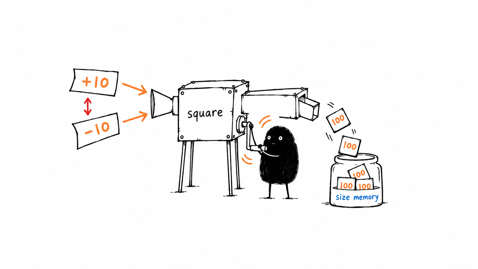
RMSProp remembers gradient size without preserving sign, so large repeated swings still produce a large denominator.

Divide by that size estimate

For each parameter:

$$w_t=w_{t-1}-\alpha \frac{g_t}{\sqrt{s_t}+ϵ}$$

The small positive number $ϵ$ prevents division by zero and limits amplification when the denominator is tiny.

Equivalently, each parameter has an effective multiplier:

$${\alpha }_{\text{effective},i,t}=\frac{\alpha }{\sqrt{s_{i,t}}+ϵ}$$

A history of large gradients produces a larger denominator. That reduces the multiplier applied to the current gradient.

A history of smaller gradients produces a smaller denominator. That increases the multiplier relative to the large-gradient parameter.

This is an adaptive update: its scaling changes during training.

What happens to gradients of 1 and 100?

Suppose those gradients remain constant long enough for the averages to settle:

$$s_1\approx 1,s_2\approx 10,000$$

Ignoring a negligible $ϵ$:

$$\frac{1}{\sqrt{1}}=1,\frac{100}{\sqrt{10,000}}=1$$

The raw gradient scale no longer creates a hundredfold difference in update magnitude in this example.

Actual training is less tidy. Gradients change, averages lag, and parameter interactions matter. RMSProp does not guarantee identical updates or a perfectly shaped loss surface.

It also does not calculate curvature directly. A large gradient can result from several causes. RMSProp uses gradient magnitude as a practical scaling signal.

See the state change

This example isolates two gradient histories. They are supplied values, not gradients from a complete training run.

import numpy as np

w = np.array([1.0, 1.0])
s = np.zeros_like(w)
alpha, beta, epsilon = 0.01, 0.9, 1e-8

gradients = [
    np.array([1.0, 100.0]),
    np.array([1.0, -100.0]),
    np.array([1.0, 100.0]),
    np.array([1.0, -100.0]),
]

for t, g in enumerate(gradients, start=1):
    # NumPy squares each entry separately.
    s = beta * s + (1 - beta) * g ** 2
    scale = np.sqrt(s) + epsilon
    step = alpha * g / scale
    w -= step

    print(f"update={t}")
    print("gradient:       ", g)
    print("squared average:", s)
    print("denominator:    ", scale)
    print("step:           ", step)
    print("weights:        ", w, "\n")

The second parameter’s denominator stays positive when its gradient reverses. Squaring removes the sign from the history; the current gradient still supplies the update’s direction.

At the first update, the averages start below their settled values because we initialized them at zero. Basic RMSProp here leaves that startup effect uncorrected.

For a network, keep a separate s array for each weight matrix and bias vector. Squaring and division are element by element, not matrix multiplication.

Final Mental Model

What this still leaves open:

RMSProp scales the current gradient. In the version above, it does not average the direction before updating.

Momentum does average direction, but does not divide by a running gradient-size estimate.

That gives us two useful pieces:

Method	Stored history	Purpose
Momentum	Signed gradients	Smooth the update direction
RMSProp	Squared gradients	Adapt the update scale

What if we used both, then corrected their zero-start bias?

That brings us to Adam.

Further reading: RMSProp in Hinton’s lecture slides.