Why Learning Rates Should Decay During Training

The model learns quickly at first. Then the loss keeps bouncing around the same range.

The optimizer is still calculating gradients. The weights are still changing. Nothing has crashed.

So why has progress slowed?

The uncomfortable answer is that the learning rate that helped us move quickly at the beginning can become too large for the work that remains near the end.

That raises the real question:

Why should the same step size be used when we are far from the minimum and when we are already close to it?

The idea in 30 seconds

Learning-rate decay does not make gradients smarter. It changes how loudly we listen to them.

Early in training, a larger learning rate helps the optimizer travel quickly through parameter space. Later, especially with mini-batch noise, the same multiplier can keep shaking the weights around a good region. Decay is the compromise: take larger steps while the signal is useful, then reduce the multiplier when noisy updates start dominating the final movement.

What is the learning rate actually doing?

For one parameter, gradient descent with a time-varying learning rate looks like:

$$w_{t+1}=w_t-{\alpha }_t{g}_t$$

Read the equation mechanically:

• $w_t$ is the current parameter value.
• $g_t$ is the gradient estimate at this update.
• ${\alpha }_t$ is the multiplier applied to that estimate.
• ${\alpha }_t{g}_t$ is the actual step.

The gradient supplies direction and magnitude. The learning rate decides how much of that signal becomes movement.

Writing ${\alpha }_t$ instead of $\alpha$ keeps one possibility open: the multiplier does not have to stay fixed.

But before we reduce it, we should be honest about what problem we are solving.

Does a constant learning rate always fail?

No.

Take the simple loss:

$$J(w)=\frac{1}{2}{w}^2$$

Its gradient is $w$, so with a constant learning rate:

$$w_{t+1}=(1-\alpha )w_t$$

For $0<\alpha <2$, this converges to zero.

That matters because it rules out a sloppy explanation:

“Learning rates must decay because otherwise gradient descent can never converge.”

That is not generally true. In this clean deterministic example, the gradient itself becomes smaller as $w$ approaches zero, so the step naturally shrinks:

$$\text{step}=\alpha w_t$$

If $w_t$ gets smaller, the step gets smaller too.

So constant learning rate is not automatically broken.

Something else has to be happening.

What changes when the gradient is noisy?

Mini-batch training changes the final stage of optimization.

Near a minimum, the full gradient can be small while individual batch gradients remain nonzero. One batch says “move a little left.” Another says “move a little right.” Neither batch is necessarily wrong; each is just a noisy estimate of the full training signal.

For the same one-parameter example, write the mini-batch gradient estimate as:

$$g_t=w_t+{\epsilon }_t$$

Here, ${\epsilon }_t$ is zero-mean gradient noise.

The update becomes:

$$w_{t+1}=(1-{\alpha }_t)w_t-{\alpha }_t{\epsilon }_t$$

This equation separates the two forces:

• $(1-{\alpha }_t)w_t$ is the part pulling the parameter toward zero.
• $-{\alpha }_t{\epsilon }_t$ is the part caused by noisy batch-to-batch variation.

Far from the minimum, $w_t$ is large, so the useful signal can dominate.

Near the minimum, $w_t$ becomes small, but ${\epsilon }_t$ does not automatically vanish. The noise term can keep moving the parameter even when the full-gradient signal is tiny.

With constant $\alpha$, independent noise of variance ${\sigma }^2$, and $0<\alpha <2$, the long-run parameter variance in this toy model is:

$$\mathrm{Var}(w)=\frac{\alpha {\sigma }^2}{2-\alpha }$$

We get this by setting:

$$V=(1-\alpha {)}^{2}V+{\alpha }^2{\sigma }^2$$

and solving for $V$.

The exact formula belongs to this simple model, not every neural network. But the mechanism is the useful part: a larger learning rate creates a higher noise floor, while a smaller learning rate reduces how much noisy gradients can shake the parameter.

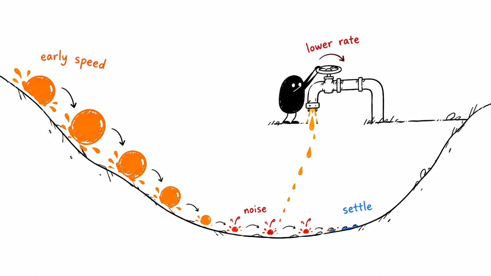
Decay keeps early movement large enough to travel, then lowers the multiplier so late noisy updates have less room to shake the parameters.

What would a good solution need to do?

We want two different behaviors from the same optimizer.

Early in training:

• the parameters may be far from a good region
• gradients often contain useful directional signal
• larger steps can reduce loss quickly

Late in training:

• the full-gradient signal may be small
• mini-batch noise can still be present
• large steps can keep the weights bouncing around

So the desired behavior is:

early training
    use a larger multiplier
    move quickly

later training
    use a smaller multiplier
    reduce noisy movement

That is the reason learning-rate decay exists.

It is not magic. It is a schedule for changing how strongly the optimizer responds to each gradient estimate.

How can the multiplier decay?

Let $e$ count completed epochs, starting at zero. Let ${\alpha }_0$ be the initial learning rate.

A learning-rate schedule is just a rule for computing $\alpha$ from some clock: epoch number, update number, validation plateau, or another signal.

Common fixed schedules include:

Schedule	Rule	Behavior
Inverse time	${\alpha }_e={\alpha }_0/(1+ke)$	Gradual decrease
Exponential	${\alpha }_e={\alpha }_0{\gamma }^e$, $0<\gamma <1$	Same fractional decrease each epoch
Step	${\alpha }_e={\alpha }_0{\gamma }^{\lfloor e/K\rfloor }$	Multiply by $\gamma$ every $K$ epochs
Cosine	${\alpha }_e={\alpha }_{\min }+\frac{1}{2}({\alpha }_0-{\alpha }_{\min })[1+\cos (\pi e/E)]$	Smooth decrease over $E$ epochs

The names describe different mathematical rules. In particular, ${\alpha }_0/(1+ke)$ is inverse-time decay, even if an assignment or code comment loosely calls it exponential decay.

For inverse-time decay, $k\ge 0$ controls how quickly the rate falls. For cosine decay, the formula is usually used over a fixed horizon $E$; extending it blindly past that horizon would raise the rate again.

Also, learning-rate decay and weight decay are different. Learning-rate decay changes the optimizer’s global step multiplier. Weight decay shrinks parameters through a separate rule or regularization mechanism.

Can we see the noise floor directly?

The small experiment below uses the same noise sequence twice.

The only difference is the learning-rate rule.

import numpy as np

rng = np.random.default_rng(7)
noise = rng.normal(0, 0.4, size=500)
alpha0 = 0.2

def train(use_decay):
    w = 3.0
    history = []

    for t, disturbance in enumerate(noise):
        # This demonstration schedules by UPDATE, not epoch.
        alpha = alpha0 / (1 + 0.02 * t) if use_decay else alpha0

        # True gradient plus sampling-like noise.
        g = w + disturbance
        step = alpha * g
        w -= step
        history.append(w)

        if t in (0, 1, 10, 100, 499):
            print(f"update={t + 1}, lr={alpha:.5f}, "
                  f"gradient={g:+.5f}, step={step:+.5f}, w={w:+.5f}")

    # Typical distance from zero over the final 100 updates.
    tail_rms = np.sqrt(np.mean(np.square(history[-100:])))
    return tail_rms

print("CONSTANT RATE")
print("final-window RMS:", train(False))
print("\nDECAYING RATE")
print("final-window RMS:", train(True))

The experiment is deliberately small. It is not proof that every decay schedule improves every neural network.

It answers one narrower question:

If the gradient estimate remains noisy near the minimum, what happens when we shrink the multiplier applied to that noise?

The answer is that the final motion usually becomes quieter. The model may still move, but the same noisy gradient produces a smaller step.

That is the behavior decay is trying to buy.

Which clock is the schedule using?

This is an easy implementation detail to get wrong.

An epoch contains many parameter updates in mini-batch training. Reducing the rate every ten epochs is not the same as reducing it every ten updates. Changing batch size also changes the number of updates per epoch.

So every schedule should make its clock explicit:

epoch-based schedule:
    alpha = f(epoch)

update-based schedule:
    alpha = f(update_number)

plateau-based schedule:
    alpha changes when validation progress stalls

Compute the scheduled rate from the initial rate and the chosen clock. Repeatedly applying a closed-form rule to the already reduced rate can accidentally compound the decay.

Adam can use a learning-rate schedule too. Adam adapts the update per parameter; the learning-rate schedule controls the global multiplier around that adaptive update.

Those are different levels of control.

What can go wrong?

Decay solves a tradeoff, so it can fail on both sides.

If the learning rate decays too quickly, the model may barely move while there is still useful learning to do. Training looks stable, but only because the optimizer has become timid.

If the learning rate stays too large, later updates can remain noisy or unstable. Training may keep improving in tiny bursts, then lose those gains to the next few batches.

The practical check is not just a smooth training curve. Use a fixed evaluation set. Watch validation loss as well as training loss. A schedule can be fixed in advance, or it can respond to a plateau.

The point is not to worship decay. The point is to make the step size match the stage of training.

Final Mental Model

Learning-rate decay exists because the optimizer’s job changes during training: early on, we want movement; later, we want settling.

The update is still the same small operation:

calculate a gradient
choose how strongly to trust it
change the weights

Decay changes the second line over time.

Across this optimizer series, we changed how much data an update sees, how much direction history it remembers, how it scales each parameter, and how the global multiplier changes over time.

The core idea is the same throughout:

Optimization is not just about knowing which way is downhill. It is about deciding how much of each imperfect signal should become movement.