Adam From First Principles

We have built two kinds of memory.

Momentum remembers which direction gradients have been pointing. RMSProp remembers how large they have been.

Adam uses both. But there is one more problem to solve before combining them: both memories start at zero.

Two questions for every parameter

Let $g_t$ be the current gradient for one neural-network parameter.

The first question is: what direction has this gradient usually pointed recently?

Keep a running average:

$$m_t={\beta }_1{m}_{t-1}+(1-{\beta }_1)g_t$$

The second question is: how large has this gradient been recently, regardless of sign?

Keep a running average of squares:

$$v_t={\beta }_2{v}_{t-1}+(1-{\beta }_2)g_t^2$$

The letters change from the previous posts to match the Adam paper. Here, $m$ holds the signed average and $v$ holds the squared average.

The two $\beta$ values control separate memory lengths.

Statistically, these estimate a first moment and a second raw moment. Those mean an average gradient and an average squared gradient. The second raw moment is not the variance; variance subtracts the square of the mean.

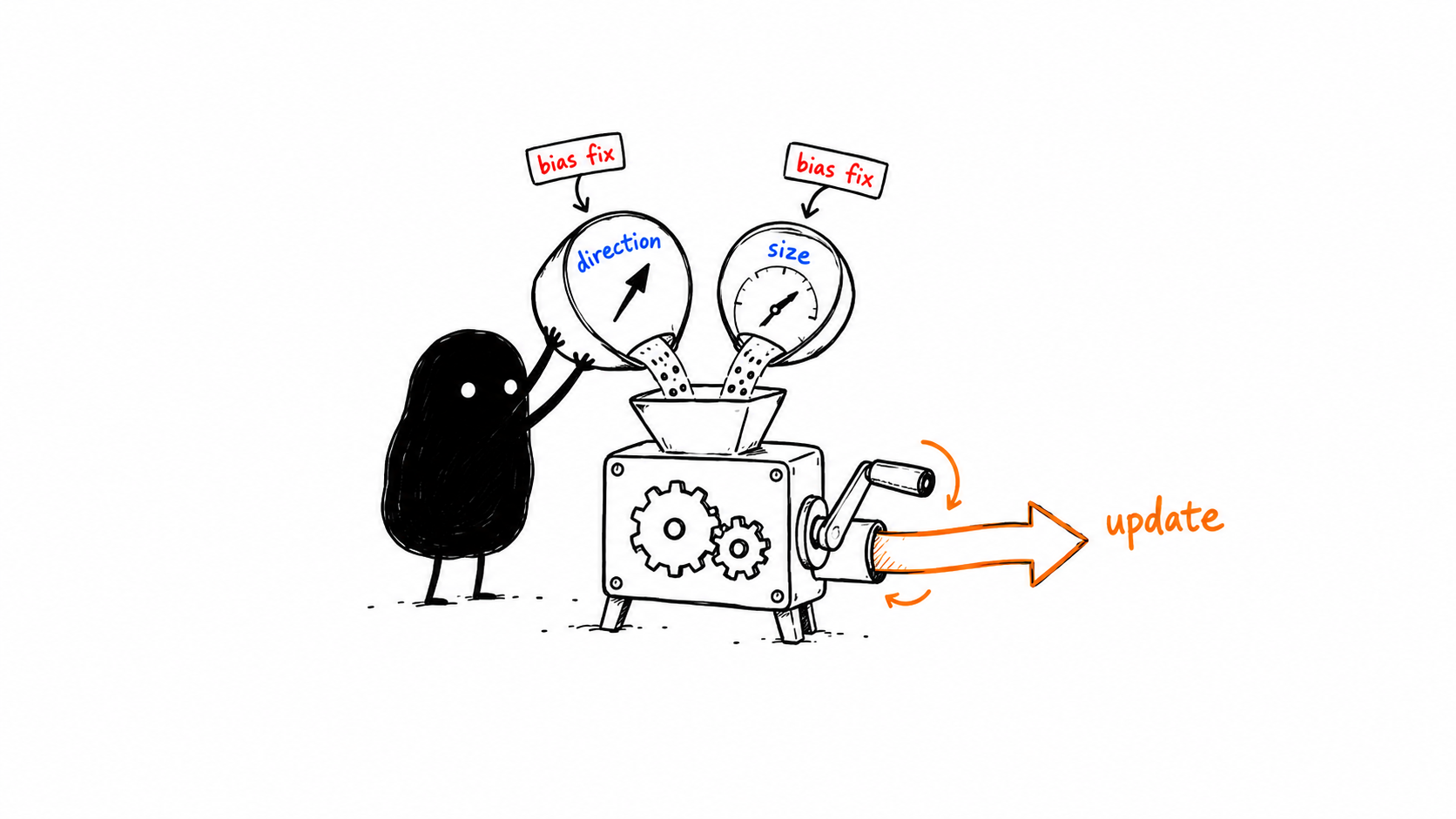
Adam is built from two memories: one for where gradients have pointed and one for how large they have been.

Why starting at zero matters

Suppose every gradient is exactly 5. Set ${\beta }_1=0.9$ and $m_0=0$.

Then:

$$m_1=0.5,m_2=0.95,m_3=1.355$$

We are trying to estimate 5, but the estimate begins much smaller.

This is not evidence that the gradients are small. It is an effect of initializing the average at zero.

For a constant gradient $g$, expand the recurrence:

$$m_t=(1-{\beta }_1)g\left(1+{\beta }_1+\cdots +{\beta }_1^{t-1}\right)$$

The geometric sum simplifies to:

$$m_t=g(1-{\beta }_1^t)$$

So divide by the missing weight:

$${\hat{m}}_t=\frac{m_t}{1-{\beta }_1^t}$$

At the first step, $0.5/(1-0.9)=5$.

Apply the same correction to the squared average:

$${\hat{v}}_t=\frac{v_t}{1-{\beta }_2^t}$$

This is bias correction. It removes the attenuation caused by the zero initialization. Under a stationary gradient distribution, it corrects the corresponding expectation. It does not remove sampling noise or make a changing gradient history perfectly current.

Now combine direction and scale

The update is:

$${\theta }_t={\theta }_{t-1}-\alpha \frac{{\hat{m}}_t}{\sqrt{{\hat{v}}_t}+ϵ}$$

Read the fraction from top to bottom.

The numerator supplies a smoothed direction. The denominator scales it using recent gradient magnitude.

The learning rate $\alpha$ still controls the overall update scale. Adam adapts updates; it does not remove the learning-rate choice.

Its name comes from adaptive moment estimation.

One complete example

This trains a linear neuron to learn $\hat{y}=2x+1$. We use full-data gradients to keep the optimizer state easy to inspect. Adam can also use mini-batch gradients.

import numpy as np

X = np.linspace(-1, 1, 20)
Y = 2 * X + 1
theta = np.array([0.0, 0.0])  # [weight, bias]
m = np.zeros_like(theta)
v = np.zeros_like(theta)
alpha = 0.05
beta1, beta2, epsilon = 0.9, 0.999, 1e-8

for t in range(1, 201):
    # Compute both derivatives BEFORE changing either parameter.
    error = theta[0] * X + theta[1] - Y
    g = np.array([np.mean(error * X), np.mean(error)])

    # Update the two persistent memories.
    m = beta1 * m + (1 - beta1) * g
    v = beta2 * v + (1 - beta2) * g ** 2

    # t counts parameter updates, starting at 1.
    m_hat = m / (1 - beta1 ** t)
    v_hat = v / (1 - beta2 ** t)
    step = alpha * m_hat / (np.sqrt(v_hat) + epsilon)
    theta -= step

    if t in (1, 2, 3, 10, 50, 100, 200):
        cost = 0.5 * np.mean((theta[0] * X + theta[1] - Y) ** 2)
        print(f"update={t}, cost={cost:.6f}")
        print("gradient:", g)
        print("m:", m, "v:", v)
        print("m_hat:", m_hat, "v_hat:", v_hat)
        print("step:", step, "[weight, bias]:", theta, "\n")

The learning rate 0.05 is chosen for this small demonstration. The original paper suggests 0.001 as a default for its tested problems, alongside ${\beta }_1=0.9$, ${\beta }_2=0.999$, and $ϵ=10^{-8}$.

For a larger network, each parameter array gets matching m and v arrays. Keep them between batches and epochs. Increment t once per optimizer update, not once for every layer.

The final weights should approach 2 and 1. More importantly, the prints show how raw gradients become corrected, scaled updates.

Final Mental Model

Adam is a rule, not a guarantee.

It does not guarantee the best validation performance, a global minimum, or successful training with any learning rate.

What it gives us is a precise way to combine two useful histories and correct their startup attenuation.

We now know how to choose an update direction and adapt its scale per parameter.

One question remains: should the overall learning rate stay the same from the first update to the last?

Further reading: Kingma and Ba, Adam: A Method for Stochastic Optimization, especially Algorithm 1 and the bias-correction derivation.