Why Gradient Descent Needs Momentum

Left. Right. Left. Right.

The loss is falling. The weights are moving. But most of that movement is across the same narrow valley.

Why does gradient descent keep changing its mind?

In the previous post, we used mini-batches to estimate the gradient cheaply. Now we need to decide what to do with those estimates over time.

A gradient describes where we are now

Let $\theta$ represent the trainable parameters of a neural network: its weights and biases.

Ordinary gradient descent uses:

$${\theta }_t={\theta }_{t-1}-\alpha g_t$$

Here, $g_t$ is the gradient at the current parameters. The index $t$ counts updates.

This rule uses the current gradient directly. It stores no separate history of earlier gradients.

That becomes expensive when the loss changes much faster in one direction than another.

Two weights are enough to see the problem

Consider a simple local model of a neural network’s loss:

$$J(w_1,w_2)=\frac{1}{2}(w_1^2+100w_2^2)$$

Its gradient is:

$$g=\left[\begin{array}{c}{w}_1\\ 100w_2\end{array}\right]$$

The loss curves sharply along $w_2$, but gently along $w_1$. Equal-loss contours are long ellipses.

With $\alpha =0.019$, ordinary gradient descent gives:

$$w_1\leftarrow 0.981w_1,w_2\leftarrow -0.9w_2$$

The first weight makes slow progress. The second changes sign every update.

Increasing the learning rate could speed up $w_1$, but it can destabilize $w_2$. One parameter limits the step we can take everywhere.

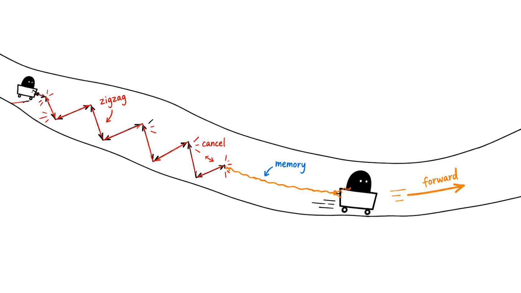
Momentum keeps useful direction from repeated gradients while letting opposing sideways motion cancel out over time.

What information survives the oscillation?

Look at two possible gradient sequences:

$$\text{consistent direction: }1,1,1,1$$ $$\text{alternating direction: }10,-10,10,-10$$

The first sequence keeps pointing the same way. The second repeatedly reverses.

We want an update that preserves consistent direction while reducing repeated reversals.

An average can do that. But storing every past gradient would cost more memory as training continues.

Instead, keep one running value:

$$v_t=\beta v_{t-1}+(1-\beta )g_t$$

This is an exponentially weighted average. The number $\beta$, between zero and one, controls how much history we retain.

With $\beta =0.9$, the new value contains 90% of the previous average and 10% of the current gradient.

Starting from zero and expanding three updates gives:

$$v_3=(1-\beta )\left(g_3+\beta g_2+{\beta }^2{g}_1\right)$$

Older gradients receive progressively smaller weights. We retain history without storing a growing list.

The rough memory scale is $1/(1-\beta )$ updates. At 0.9, that is about ten updates, not a strict ten-step window.

Use that average to update the weights

Momentum, in the averaging convention used here, becomes:

$$v_t=\beta v_{t-1}+(1-\beta )g_t$$ $${\theta }_t={\theta }_{t-1}-\alpha v_t$$

Consistent gradients reinforce the running direction. Opposing gradients partly cancel.

Cancellation is not perfect. Momentum can still oscillate, and its history can carry it past a minimum. It needs a suitable learning rate.

Also, many implementations use:

$$u_t=\beta u_{t-1}+g_t$$

They omit the factor $(1-\beta )$. Starting from zero, $v_t=(1-\beta )u_t$. Matching the updates requires scaling the learning rate accordingly. Using identical learning-rate values does not give identical algorithms.

A small experiment

import numpy as np

def gradient(w):
    # Derivative of 0.5 * (w1**2 + 100 * w2**2).
    return np.array([w[0], 100 * w[1]])

def cost(w):
    return 0.5 * (w[0] ** 2 + 100 * w[1] ** 2)

plain = np.array([2.0, 2.0])
momentum = plain.copy()
velocity = np.zeros_like(momentum)
alpha, beta = 0.019, 0.9

for t in range(1, 101):
    plain -= alpha * gradient(plain)

    g = gradient(momentum)
    # Keep the state between updates. Do not reset it here.
    velocity = beta * velocity + (1 - beta) * g
    momentum -= alpha * velocity

    if t in (1, 2, 3, 10, 50, 100):
        print(f"update={t}")
        print("plain:   ", plain, "cost:", cost(plain))
        print("momentum:", momentum, "cost:", cost(momentum))
        print("average: ", velocity, "\n")

Both methods begin at the same point and use the same averaging-convention learning rate. This demonstrates their paths; it does not establish that Momentum always wins at identical hyperparameters. Each method can require different tuning.

In a full network, every weight and bias gets its own running average, with the same shape as that parameter.

Final Mental Model

Momentum gives the update a memory of direction.

But direction is only part of the problem. Different parameters can still have very different gradient scales.

Can we adjust the step for each parameter separately?

Further reading: Hinton’s optimization lectures.