Why Mini-Batch Gradient Descent Works

One million training examples. One weight update.

That is what full-batch gradient descent asks us to do: read the entire training set before changing a single parameter.

But do we really need every example to decide which way to move?

In the previous post, we looked at input normalization. It makes the optimization problem easier to navigate. Now there is another problem: how much work should we do before taking each step?

Start with one neuron

Take a neuron with one input, one weight, and one bias:

$${\hat{y}}_i=w{x}_i+b$$

For now, use squared error. The loss for one example is:

$${\ell }_i=\frac{1}{2}({\hat{y}}_i-y_i{)}^2$$

For $N$ examples, the cost is their average:

$$J(w,b)=\frac{1}{N}\sum _{i=1}^N{\ell }_i$$

A gradient tells us how this cost changes when we change a parameter slightly. For the weight:

$$\frac{\partial J}{\partial w}=\frac{1}{N}\sum _{i=1}^N({\hat{y}}_i-y_i)x_i$$

Notice what we are computing. Each example contributes one value. We average those values, then update the weight:

$$w\leftarrow w-\alpha \frac{\partial J}{\partial w}$$

Here, $\alpha$ is the learning rate. It controls the size of the update.

The question is whether we need the complete average every time.

Three ways to take a step

Batch gradient descent uses all $N$ examples for each update. Its gradient is exact for the current training-set objective, assuming deterministic computation.

Stochastic gradient descent, in the single-example sense, uses one example. We update immediately, but that example may be a poor guide to the whole dataset.

Mini-batch gradient descent uses a group of $B$ examples. It sits between those two choices. In practice, people also use “SGD” to describe mini-batch training.

Method	Examples per update	Updates per epoch
Full batch	$N$	1
Single-example SGD	1	$N$
Mini-batch	$B$	$\lceil N/B\rceil$

An epoch means one pass through the training set. An update means one change to the parameters. They are different clocks.

With 1,000 examples and a batch size of 64, an epoch contains 16 updates. The last batch contains 40 examples.

Why an incomplete gradient can still work

Suppose the current weight is too small. Most examples may push it upward, although some push it downward.

A randomly selected group can still reveal that overall direction.

For a uniformly sampled batch, at fixed parameters, the batch-average gradient is an unbiased estimate of the full gradient:

$$\mathbb{E}[g_B]=g_{\text{full}}$$

“Unbiased” means correct on average over the sampling process. It does not mean every batch points in the correct direction.

Write the batch gradient as:

$$g_B=g_{\text{full}}+{\epsilon }_B$$

The extra term is sampling noise: the difference caused by which examples we selected.

For independent samples, averaging $B$ gradients reduces their variance by a factor of $B$. The typical noise size therefore scales as $1/\sqrt{B}$. Sampling without replacement adds a finite-population correction.

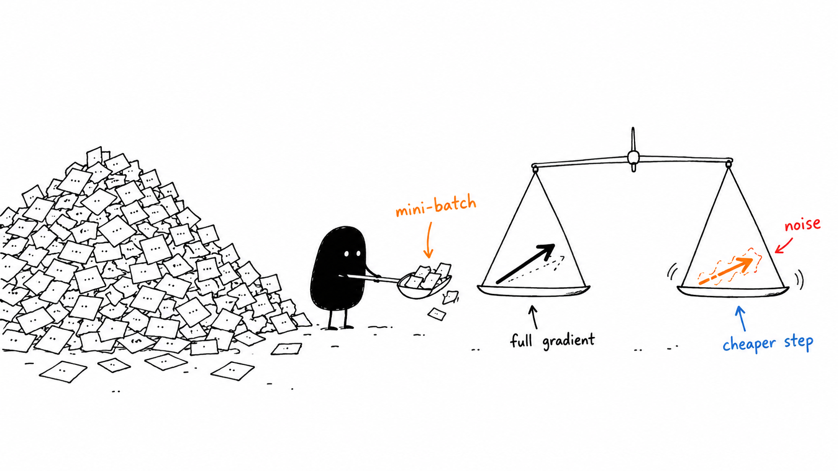
A mini-batch is useful when its noisy estimate preserves enough of the full dataset’s direction to justify a cheaper update.

So a batch of 64 generally gives a steadier estimate than one example. It still costs less per update than reading the entire dataset.

There is a detail here: shuffling once per epoch samples without replacement. After earlier batches change the weights, the remaining batch is not a fresh independent sample at those new weights. The unbiasedness statement describes the sampling setup above, not every conditional step of a shuffled training run.

Watch it happen in NumPy

This trains a single linear neuron. We keep every gradient visible.

import numpy as np

rng = np.random.default_rng(7)
X = np.linspace(-1, 1, 10)  # Ten input examples.
Y = 2 * X + 1              # Target: weight 2, bias 1.
w, b = 0.0, 0.0
learning_rate = 0.1
batch_size = 4

for epoch in range(3):
    # Apply the SAME permutation to inputs and targets.
    order = rng.permutation(len(X))

    for start in range(0, len(X), batch_size):
        ids = order[start:start + batch_size]
        xb, yb = X[ids], Y[ids]
        error = w * xb + b - yb

        # mean() uses the actual size, including the last batch.
        dw = np.mean(error * xb)
        db = np.mean(error)
        w -= learning_rate * dw
        b -= learning_rate * db

        print(f"epoch={epoch}, size={len(ids)}, "
              f"dw={dw:+.4f}, db={db:+.4f}, "
              f"w={w:.4f}, b={b:.4f}")

    # Evaluate the SAME full dataset after each epoch.
    cost = 0.5 * np.mean((w * X + b - Y) ** 2)
    print(f"full_dataset_cost={cost:.6f}\n")

Each epoch has batches of 4, 4, and 2. Change batch_size to 1 or 10 to see the other two methods.

Batch losses can rise simply because the next batch contains harder examples. Comparing loss on a fixed dataset gives a clearer view of progress.

Then why not always use the smallest batch?

One example gives frequent updates, but frequent is not automatically efficient.

Hardware can process groups of examples together using matrix operations. Very small batches may leave that capacity underused. Larger batches also require more memory and provide fewer updates per epoch.

The useful comparison is therefore time, memory, and validation performance together. A smooth training curve alone does not choose the best batch size.

Final Mental Model

Mini-batch gradient descent works because we can learn from an estimate before calculating the complete answer.

But the estimate changes from batch to batch. What if we remembered recent gradients instead of reacting to each one independently?

That is where Momentum starts.

Further reading: Hinton’s neural-network optimization lectures.