Why Deep Neural Networks Become Hard to Train: Vanishing Gradients, Exploding Gradients, and Weight Initialization

In the previous post, we looked at regularization through the lens of gradient descent.

We started with the update rule

$$W:=W-\alpha dW$$

and then asked what changes when we deliberately constrain the learning process using techniques such as L2 regularization and dropout.

But there is another problem hiding inside this equation.

The update rule assumes that $dW$ is actually useful.

What happens if the gradient becomes almost zero?

Or what happens if it becomes enormous?

That takes us to one of the fundamental optimization problems in deep neural networks:

Vanishing and exploding gradients.

---

1. Where does the gradient come from?

Consider a deep network:

$$X\to A^{[1]}\to A^{[2]}\to A^{[3]}\to A^{[4]}\to \hat{Y}$$

During forward propagation, information moves from the input toward the output.

During backpropagation, the gradient travels in the opposite direction:

$$\hat{Y}\to A^{[4]}\to A^{[3]}\to A^{[2]}\to A^{[1]}$$

Suppose we want to update the weights in the first layer.

The network needs to answer:

If I slightly change $W^{[1]}$, how does the final loss change?

Mathematically:

$$\frac{\partial J}{\partial W^{[1]}}$$

The difficulty is that $W^{[1]}$ affects the loss through every layer after it.

So by the chain rule, the gradient contains many multiplied terms.

Schematically:

$$\frac{\partial J}{\partial W^{[1]}}=\frac{\partial J}{\partial A^{[L]}}\frac{\partial A^{[L]}}{\partial A^{[L-1]}}\frac{\partial A^{[L-1]}}{\partial A^{[L-2]}}\cdots \frac{\partial A^{[1]}}{\partial W^{[1]}}$$

The important observation is not the exact expression.

It is this:

$$\boxed{\text{Backpropagation repeatedly multiplies derivatives}}$$

And repeated multiplication can behave very differently depending on the numbers involved.

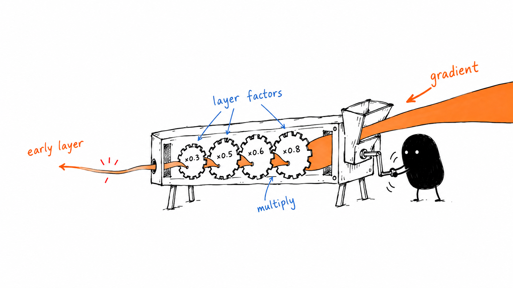
Backpropagation does not pass a gradient back unchanged; each layer contributes another multiplication factor on the way to earlier weights.

---

2. What if those numbers are smaller than 1?

Imagine, just for intuition, that each layer contributes a factor of approximately:

$$0.5$$

With two layers:

$$0.5^2=0.25$$

With five layers:

$$0.5^5=0.03125$$

With twenty layers:

$$0.5^{20}\approx 9.5\times 10^{-7}$$

The gradient has almost disappeared.

So an early-layer gradient might become:

$$d{W}^{[1]}\approx 0$$

Then gradient descent performs:

$$W^{[1]}:=W^{[1]}-\alpha d{W}^{[1]}$$

If

$$d{W}^{[1]}\approx 0$$

then:

$$W_{\text{new}}^{[1]}\approx W_{\text{old}}^{[1]}$$

The weights barely move.

This is the vanishing gradient problem.

The early layers of a deep network can learn extremely slowly because the learning signal becomes weaker and weaker as it travels backward.

---

3. What if the multiplied values are larger than 1?

Now suppose each layer contributes roughly:

$$2$$

After twenty layers:

$$2^{20}=1,048,576$$

Instead of disappearing, the gradient becomes enormous.

Suppose:

$$dW=100000$$

and:

$$\alpha =0.01$$

Then:

$$\Delta W=-\alpha dW=-1000$$

A single gradient update can move a parameter by a huge amount.

Training may become unstable.

The loss can oscillate wildly or even become NaN.

This is the exploding gradient problem.

So the two extremes are:

$$\boxed{|dW|\to 0}\text{Vanishing gradient}$$

and

$$\boxed{|dW|\to \text{very large}}\text{Exploding gradient}$$

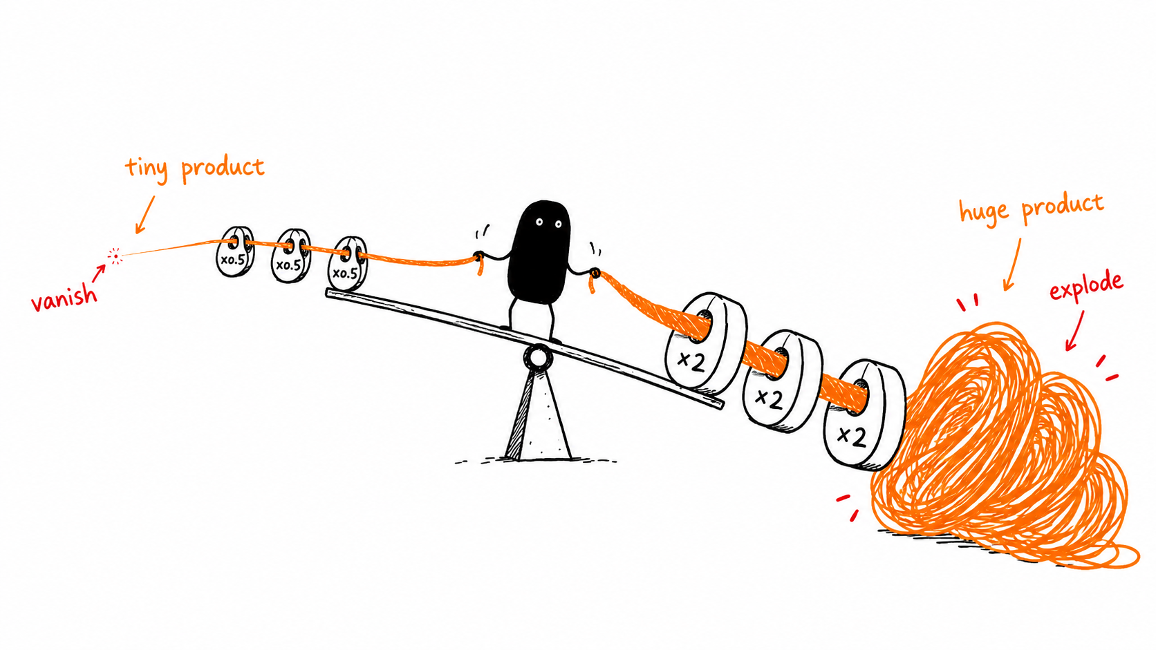
Products below one can fade into an almost useless learning signal, while products above one can turn the same update rule unstable.

---

4. Where do these repeated factors come from?

Consider one layer:

$$Z^{[l]}=W^{[l]}{A}^{[l-1]}+b^{[l]}$$

and:

$$A^{[l]}=g(Z^{[l]})$$

During backpropagation, we compute:

$$d{Z}^{[l]}=d{A}^{[l]}\odot g^{\prime }(Z^{[l]})$$

and then:

$$d{A}^{[l-1]}=(W^{[l]}{)}^{T}d{Z}^{[l]}$$

So every layer introduces factors involving:

1. the weight matrix
2. the derivative of the activation function

This is important.

Gradient flow is not determined by the activation function alone.

It depends on a chain involving both:

$$W^{[l]}$$

and

$$g^{\prime }(Z^{[l]})$$

across many layers.

---

5. Why is sigmoid particularly problematic?

The sigmoid function is:

$$\sigma (z)=\frac{1}{1+e^{-z}}$$

Its derivative is:

$${\sigma }^{\prime }(z)=\sigma (z)(1-\sigma (z))$$

The maximum possible derivative is:

$$0.25$$

And when $z$ becomes very positive or very negative:

$${\sigma }^{\prime }(z)\approx 0$$

For example:

$$z\gg 0\Rightarrow \sigma (z)\approx 1$$

therefore:

$${\sigma }^{\prime }(z)\approx 1(1-1)=0$$

Similarly:

$$z\ll 0\Rightarrow \sigma (z)\approx 0$$

and again:

$${\sigma }^{\prime }(z)\approx 0$$

This region is often called the saturated region of sigmoid.

During backpropagation:

$$dZ=dA\cdot {\sigma }^{\prime }(Z)$$

If:

$${\sigma }^{\prime }(Z)\approx 0$$

then:

$$dZ\approx 0$$

And this small gradient is then passed to the previous layer.

If several layers behave this way:

$$\text{small}\times \text{small}\times \text{small}\times \cdots$$

the gradient can disappear.

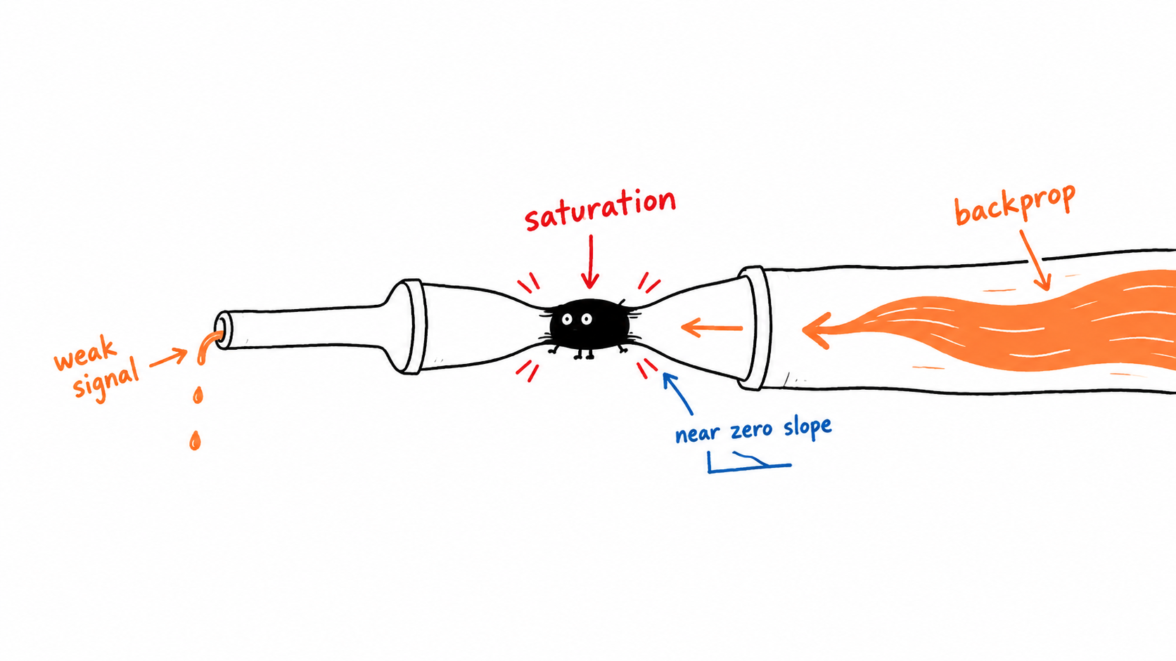
A saturated activation behaves like a pinched pipe: the incoming gradient may be present, but the local derivative lets very little through.

---

6. What about tanh?

The hyperbolic tangent activation is:

$$\tanh (z)$$

with derivative:

$${\tanh }^{\prime }(z)=1-{\tanh }^2(z)$$

Around:

$$z\approx 0$$

its derivative can be close to:

$$1$$

which is better than sigmoid.

But when $|z|$ becomes large:

$$\tanh (z)\to \pm 1$$

and therefore:

$${\tanh }^{\prime }(z)\to 0$$

So tanh can also suffer from saturation and vanishing gradients.

---

7. Why did ReLU help?

ReLU is defined as:

$$\text{ReLU}(z)=\max (0,z)$$

Its derivative is:

$${\text{ReLU}}^{\prime }(z)=\{\begin{array}{ll}1& z>0\\ 0& z<0\end{array}$$

For positive values:

$$g^{\prime }(z)=1$$

So the gradient is not multiplied by something like:

$$0.25$$

or:

$$0.01$$

Instead:

$$dZ=dA$$

for the positive region.

This dramatically improves gradient propagation compared with sigmoid in deep networks.

But ReLU does not magically eliminate all gradient problems.

Why?

Because the weights are still involved.

Recall:

$$d{A}^{[l-1]}=(W^{[l]}{)}^{T}d{Z}^{[l]}$$

Even if:

$$g^{\prime }(z)=1$$

we are still repeatedly multiplying by weight matrices.

If the weights are too small, gradients can shrink.

If the weights are too large, gradients can explode.

That leads directly to another question:

How should we choose the initial weights of a deep neural network?

---

8. Why not initialize all weights to zero?

Suppose every neuron in a layer starts with:

$$W=0$$

Then every neuron receives the same input and produces the same output.

During backpropagation, they also receive identical gradients.

So after one update, they remain identical.

After another update, they are still identical.

The neurons fail to learn different features.

This is called the symmetry problem.

Therefore:

$$\boxed{\text{weights must start differently}}$$

This is why we initialize them randomly.

But random initialization introduces another question.

How large should those random numbers be?

---

9. Why does the scale of initialization matter?

Consider:

$$Z^{[l]}=W^{[l]}{A}^{[l-1]}$$

Suppose every weight is large.

Then $Z$ may become large.

That produces large activations, which then enter the next layer.

The process repeats:

$$\text{large activations}\to \text{large }Z\to \text{large activations}\to \cdots$$

The signal can explode as it travels forward.

The reverse can happen with very small weights.

Activations gradually shrink:

$$\text{small}\to \text{smaller}\to \text{smaller}\to \cdots$$

The same type of behavior can appear during backpropagation.

So initialization needs to achieve something subtle:

Keep the scale of activations and gradients reasonably stable as they pass through many layers.

---

10. Xavier initialization

For activation functions such as tanh, a common initialization is Xavier initialization, also called Glorot initialization.

A simplified form is:

$$W^{[l]}\sim \mathcal{N}\left(0,\frac{1}{n^{[l-1]}}\right)$$

where:

$$n^{[l-1]}$$

is the number of neurons feeding into the current layer.

In NumPy:

W = np.random.randn(n_l, n_prev) * np.sqrt(1 / n_prev)

The scaling factor is:

$$\sqrt{\frac{1}{n_{\text{prev}}}}$$

Why divide by the number of incoming neurons?

Because each neuron computes a sum:

$$z=w_1{a}_1+w_2{a}_2+\cdots +w_n{a}_n$$

As $n$ increases, more terms are being added together.

If the variance of the weights stayed fixed, the variance of $z$ would tend to increase as the number of inputs increased.

Scaling the weights based on:

$$n_{\text{in}}$$

helps counteract that growth.

The goal is approximately:

$$\text{Var}(A^{[l]})\approx \text{Var}(A^{[l-1]})$$

rather than letting activation variance continuously grow or shrink.

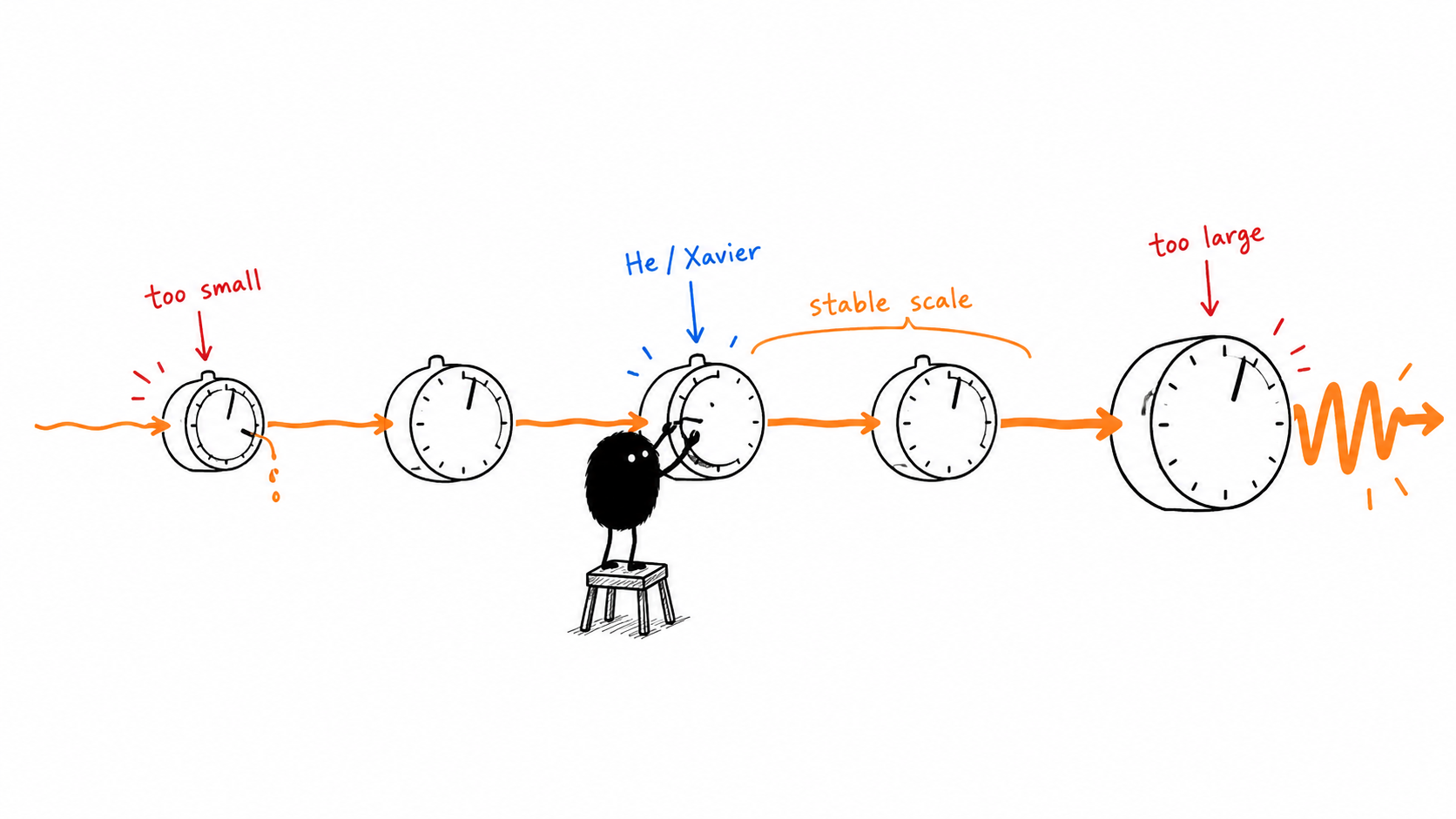
Initialization is less about making weights generically small and more about keeping the signal scale stable as it moves across layers.

---

11. Why does ReLU use a different initialization?

ReLU has an important property:

$$\text{ReLU}(z)=0\text{for }z<0$$

If the input distribution is roughly symmetric around zero, a substantial fraction of activations become zero.

So compared with an activation that preserves both positive and negative values, ReLU effectively removes part of the signal.

To compensate, we use a slightly larger initialization variance.

This leads to He initialization, introduced for rectifier networks.

The common form is:

$$W^{[l]}\sim \mathcal{N}\left(0,\frac{2}{n^{[l-1]}}\right)$$

In NumPy:

W = np.random.randn(n_l, n_prev) * np.sqrt(2 / n_prev)

The scaling factor is:

$$\boxed{\sqrt{\frac{2}{n_{\text{prev}}}}}$$

Compare that with Xavier:

$$\text{Xavier:}\sqrt{\frac{1}{n_{\text{prev}}}}$$

and:

$$\text{He:}\sqrt{\frac{2}{n_{\text{prev}}}}$$

A useful rule of thumb is:

$$\boxed{\text{tanh}\to \text{Xavier initialization}}$$

and:

$$\boxed{\text{ReLU}\to \text{He initialization}}$$

---

12. What exactly are we trying to preserve?

It is tempting to think weight initialization is simply about choosing “small enough” weights.

That is not quite right.

The real objective is to avoid systematic growth or shrinkage of the signal as depth increases.

Ideally:

$$\text{Var}(A^{[1]})\approx \text{Var}(A^{[2]})\approx \text{Var}(A^{[3]})\approx \cdots$$

and similarly during backpropagation:

$$\text{Var}(d{A}^{[L]})\approx \text{Var}(d{A}^{[L-1]})\approx \cdots$$

Not exactly.

But approximately enough that information can travel through a deep network without disappearing or exploding.

This gives us the central idea:

$$\boxed{\text{Good initialization tries to preserve signal scale across depth}}$$

---

13. A small experiment

We can see the idea with a simple NumPy experiment.

Suppose we repeatedly pass activations through many linear layers.

import numpy as np

np.random.seed(42)

n = 100
layers = 20

A = np.random.randn(n, 1000)

for l in range(layers):
    W = np.random.randn(n, n)

    Z = W @ A
    A = np.maximum(0, Z)

    print(
        f"Layer {l + 1:2d} | "
        f"mean={A.mean():.4f} | "
        f"std={A.std():.4f}"
    )

Without appropriate scaling, the activation magnitude can grow rapidly.

Now change the weight initialization to:

W = np.random.randn(n, n) * np.sqrt(2 / n)

This is He initialization.

Run the same experiment again.

The activation scale should remain much more stable across depth.

That difference is exactly what the initialization is trying to achieve.

---

14. Weight initialization does not solve everything

Even good initialization only determines where optimization starts.

After training begins, weights change.

A network can still encounter:

• unstable gradients
• poorly chosen learning rates
• saturated activations
• dead ReLU neurons
• badly scaled inputs
• optimization difficulties

Modern deep networks therefore combine several ideas:

$$\text{initialization}+\text{activation choice}+\text{normalization}+\text{optimization}+\text{architecture}$$

Later techniques such as Batch Normalization, residual connections, normalization layers, and carefully designed architectures all attack different parts of the same underlying problem:

How do we make information and gradients flow reliably through very deep networks?

---

15. Connecting everything together

The full conceptual chain is:

$$\text{Deep network}$$ $$\downarrow$$ $$\text{Backpropagation through many layers}$$ $$\downarrow$$ $$\text{Repeated multiplication of weights and derivatives}$$ $$\downarrow$$ $$\{\begin{array}{ll}\text{products become tiny}& \to \text{vanishing gradients}\\ \text{products become huge}& \to \text{exploding gradients}\end{array}$$

Activation functions influence this because:

$$dZ=dA\cdot g^{\prime }(Z)$$

Sigmoid and tanh can produce:

$$g^{\prime }(Z)\approx 0$$

in saturated regions.

ReLU improves gradient flow for:

$$Z>0$$

because:

$$g^{\prime }(Z)=1$$

But weights still control signal magnitude.

Therefore we carefully initialize them.

For tanh:

$$\boxed{W\sim \mathcal{N}\left(0,\frac{1}{n_{\text{in}}}\right)}$$

For ReLU:

$$\boxed{W\sim \mathcal{N}\left(0,\frac{2}{n_{\text{in}}}\right)}$$

---

Final Mental Model

Vanishing and exploding gradients are not mysterious bugs.

They are a natural consequence of repeatedly multiplying quantities during backpropagation.

If those quantities systematically have magnitude below $1$:

$$\text{gradient}\to \text{smaller}\to \text{smaller}\to 0$$

If they systematically have magnitude above $1$:

$$\text{gradient}\to \text{larger}\to \text{larger}\to \infty$$

Good activation functions and good initialization try to keep the network in the middle:

$$\boxed{\text{signals neither disappear nor explode}}$$

And this is one of the central ideas behind making deep neural networks trainable.

---

Papers Worth Reading

If you want to go beyond this intuition, two foundational papers connect directly to the ideas discussed here.

Xavier / Glorot Initialization

Xavier Glorot and Yoshua Bengio — Understanding the Difficulty of Training Deep Feedforward Neural Networks (2010)

This paper studies why deep networks can be difficult to optimize and develops the initialization strategy now commonly called Xavier or Glorot initialization.

He Initialization

Kaiming He, Xiangyu Zhang, Shaoqing Ren, and Jian Sun — Delving Deep into Rectifiers: Surpassing Human-Level Performance on ImageNet Classification (2015)

This work analyzes rectifier networks and introduces the initialization strategy now commonly known as He or Kaiming initialization.

---

What’s Next?

Initialization helps us control the scale of activations at the beginning of training.

But another question naturally follows:

What if the input features themselves exist on wildly different scales before they even enter the network?

For example:

$$x_1\sim 1\text{–}5$$

while:

$$x_2\sim 1000\text{–}5000$$

That leads to the next topic:

Why Normalizing Inputs Makes Gradient Descent Faster.